Linear Regression

Regression is a procedure to determine the statistical connection between a dependent variable and one or more independent variables. The variation independent variable is related with the change in the independent variables. This can be broadly classified into two main types.

1. Linear Regression
2. Logistic Regression

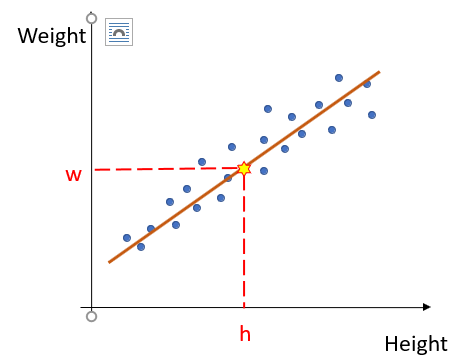
• Consider the scatter plot of the Weight vs. Height of adults as shown above.
• The trend or the form of the relationship is strongly positive.
• Now suppose we wish to estimate the weight of a person just by knowing his/ her height.
• In order to do so we first fit a straight line through our data points.
• Then from the graph, knowing the height we can find the weight of the corresponding persons.
• Hence, we are intending to find out the equation of the straight line that best describes the relationship between Weight and Height.
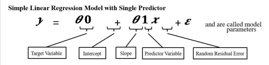
• There is only one predictor/input variable (Height) and one target variable (Weight) and we are intending to find out a relationship of the form.

y= θ0+ θ1 x

Here, y is the target variable and is the predictor variable.

We have to find out θ0 and θ1, such that the straight-line y= θ0+ θ1 x fits into our datasets best. This is called Simple Linear Regression, because it has only one predictor variable and the relationship among target and predictor variable is linear.

We use our sample data to find estimates for the coefficients/ model parameters θ_0 and θ_1 i.e.: (θ0) Ì‚ and (θ1) Ì‚.We can then predict what the value of y should be corresponding to a particular value for x by using the Least Squares Prediction Equation (also known as our hypothesis function):

y Ì‚=(θ0) Ì‚+(θ1) Ì‚x Where y Ì‚ is our prediction for y

Residuals and Residual Sum of Squares:

• For ith sample ⟨xi , y_i ⟩the predicted value of yiis (yi) Ì‚, Which we obtain from the equation (yi) Ì‚=(θ0) Ì‚+(θ1) Ì‚xi
• Then, ei=yi – (yi) Ì‚(actual – predicted) represents the ith residual.
• We define Residual Sum of Squares (RSS) as:

RSS = ∑_(i=1)^mâ–’ei2 = ∑_(i=1)^mâ–’(yi – (yi) Ì‚ )2  =  ∑_(i=1)^m▒〖(yi -((θ0) Ì‚+(θ1) Ì‚xi〗))2

There are total m no. of samples.

Mean Square Error Cost Function:

• We can define the cost function as: 

J((θ0) Ì‚,(θ1) Ì‚ )=  1/2  RSS/(Number of training samples)   =  1/2m∑_(i=1)^m▒〖(yi -((θ0) Ì‚+(θ1) Ì‚xi〗))2

Here a factor 1/2  is multiplied just for computational simplicity. Otherwise, the cost function J((θ0) Ì‚,(θ1) Ì‚ )is nothing but mean or average of the Residual sum of squares.(also known as Mean Square Error (MSE)).

Our Objective:

To find the suitable values of (θ0) Ì‚ and (θ1) Ì‚ such that the cost function J((θ0) Ì‚,(θ1) Ì‚ )   is minimized, in other words the Residual Sum of Square (RSS) is minimized. Then the straight-line y Ì‚=(θ0) Ì‚+(θ1) Ì‚x will fit our data best. This is called least squares fit.

Intuition of Cost Function:

Consider the example of single predictor variable where the hypothesis function is y Ì‚=(θ0) Ì‚+(θ1) Ì‚x and the cost function is J((θ0) Ì‚,(θ1) Ì‚ )=1/2m ∑_(i=1)^m▒〖(yi -((θ0) Ì‚+(θ1) Ì‚xi〗))2. Now we keep one parameter fixed and vary other. Let’s see how J((θ0) Ì‚,(θ1) Ì‚ ) varies.

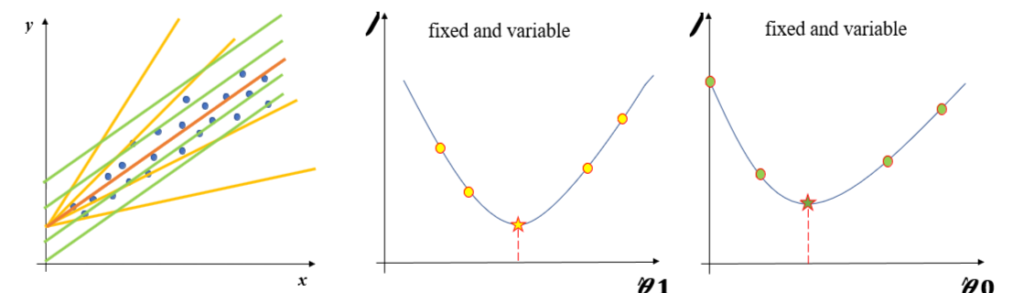
Our objective is to find the values of the parameters for which the cost function is minimized.

Solving for the best fit: Ordinary Least Squares (OLS) Regression:

• We have to Minimize RSS or J((θ0) Ì‚,(θ1) Ì‚ )  with respect to  (θ0) Ì‚” and ” (θ1) Ì‚
• Hence, we have to do, ∂/(∂(θ0) Ì‚) (RSS)=0 and ∂/(∂(θ1) Ì‚) (RSS)=0
• By solving the above two equations we get the following value of (θ1) Ì‚ and (θ0) Ì‚” “:

(θ_1 ) Ì‚=  (∑_(i=1)^m▒〖(xi – x Ì… )(y_i  – y Ì…)〗)/(∑_(i=1)^mâ–’(xi – x Ì… )2)  =r_xy   σ_y/σ_x      and    (θ0) Ì‚“ = ” y Ì…  – (θ_1 ) Ì‚x Ì…

where, x Ì…  is the mean of predictor variable x and y Ì…  is the mean of target variable y

σ_x  is the standard deviation of x and σ_y  is the standard deviation of y

and rxy is the correlation coefficient between x and y.