Multiple Linear Regression

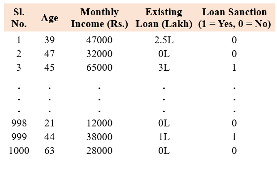
Problem Statement:

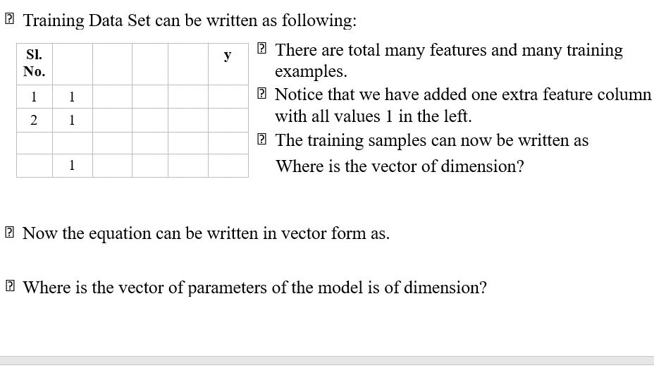
Suppose there are k many features or predictor variables x1, x2, x3, … , xk and a target variable y. Now we want to express y as a linear combination of those predictor variables. We have a vector of features/predictors x âƒ—=[x1, x2, x3, … , xk]T 

Model Representation:

Here, we can express our multiple linear regression problem by means of following probabilistic model.  y=〖 θ_0+θ〗_1 x1+θ_2  x2+θ_3  x3+…+ θ_k  x_k+ε

Here we have a vector of model parameters Θ=[〖θ_0, θ〗_1, θ_2, . . . , θ_k ]T of dimension k+1 and ε is the random error.

Like in case of simple linear regression, here also we shall use our sample data to estimate model parameter vector Θ i.e.: Θ Ì‚.

Multiple Linear Regression Assumptions:

• The predictors should be uncorrelated and linearly independent of one another.
• The model’s error term should have constant variance.
• The error term is preferably normally distributed with zero mean.

Hypothesis Function:

The predicted value of the target variable is obtained from the estimated model parameter as: 

y Ì‚=(θ0) Ì‚+(θ1) Ì‚x_1+(θ_2 ) Ì‚x_2+…+(θ_k ) Ì‚x_k=(θ0) Ì‚+∑_(j=1)^k▒〖(θ_j ) Ì‚x_j 〗

Cost Function:

Here, we shall define cost function in the following way:

(Here ⟨x âƒ—(i), y(i)⟩ is the ith data sample and y Ì‚(i) is the corresponding output of the model)

Our Objective:

To estimate the model parameters Θ Ì‚  =[(θ0) Ì‚, (θ1) Ì‚, (θ2) Ì‚  , … , (θk) Ì‚ ]T from the given sample of data so that the cost function J(Θ Ì‚ ) is minimized.

Gradient Descent algorithm for Cost Function optimization:

Gradient Descent algorithm is an optimization technique for minimizing the cost function J (Θ Ì‚)

Gradient Descent is an iterative algorithm and, in a nutshell, it does the following:

•Start with some initial values of Θ Ì‚  =[(θ0) Ì‚, (θ1) Ì‚, (θ2) Ì‚  , … , (θk) Ì‚ ]T •

•Keep Changing (θ0) Ì‚, (θ1) Ì‚, (θ2) Ì‚  , … , (θk) Ì‚ to reduce J(Θ Ì‚ )  until we end up at a minimum.

Algorithm: Gradient Descent

•Input: Feature set (X=〖[x âƒ—^((i))]〗_(i=1)^m) and corresponding values of target variable (Y= 〖[y^((i))]〗_(i=1)^m). •

•Output: Model parameters Θ Ì‚  =[(θ0) Ì‚, (θ1) Ì‚, (θ2) Ì‚  , … , (θk) Ì‚ ]T for which the cost function J(Θ Ì‚ ) is minimum. •

•Initialisation: Initialise the model parameters Θ Ì‚  =[(θ0) Ì‚, (θ1) Ì‚, (θ2) Ì‚  , … , (θk) Ì‚ ]T  with random values iteration number: t ←1

•Repeat until convergence { •Compute the cost function J(Θ Ì‚ ) •(θ_j ) Ì‚(t+1)=(θ_j ) Ì‚(t) -α ∂/(∂(θj) Ì‚ ) (J(Θ Ì‚ )), simultaneously update for every j=0,1,2,…., k •t ←t+1      }

Workshop in Probability and Statistics

Intuition of Gradient Descent algorithm:

The plot of cost function with any of the parameters (considering the other parameters fixed) is of the following form.

Now as per gradient descent rule: (θ_j ) Ì‚(t+1)=(θ_j ) Ì‚(t) -α ∂/(∂(θj) Ì‚ ) (J(Θ Ì‚ ))

Now if the gradient ∂J/(∂(θj) Ì‚) is positive, then the update in the value of (θ_j ) Ì‚ which is calculated as ” ” (θ_j ) Ì‚(t+1)” –” (θ_j ) Ì‚(t) is negative. Indicating that, in the next update (θ_j ) Ì‚ would be smaller than its previous value.

On the other hand if the gradient ∂J/(∂(θj) Ì‚) is negative, then the update in the value of (θ_j ) Ì‚ is positive. Indicating that, in the next update (θ_j ) Ì‚ would be greater than its previous value.

• The Cost Function for Linear Regression with multiple predictor variable is:

• We can calculate the derivative of the cost function with respect to (θ0) Ì‚ and (θj) Ì‚ (for j=1,2,3,…,k) as  following:

• Hence, the update rule in Gradient descent algorithm would be (for tth iteration):

for j=1,2,3,…, k

Note:

If we consider another predictor x_0 whose value is always 1 (i.e. x_0^((i) )=1, ∀i), then we can use the last equation as a generalized gradient descent update rule.

Stopping criteria for gradient descent:

We can consider following two methods as stopping criteria for the gradient descent algorithm.

1. Convergence of the model parameters:

If in two successive iterations the change in the model parameters is not significant then we can say that the algorithm has converged. As the model parameters are vectors, to compare the values of the model parameters in two successive iterations we can either take norm or absolute differences. Alternatively, if at least one of the parameters is not converged then we keep on running the algorithm until all the parameters are converged.

 2. Predefined number of iterations:

We run the algorithm for predefined number of iterations.

• How to check whether gradient descent is working or not:

We can plot cost function versus number of iterations. If it’s continuously decreasing then we can say that gradient descent is working. However, we may have to fine-tune the value of “learning rate” (α) depending upon how fast or slow the cost function is converging.

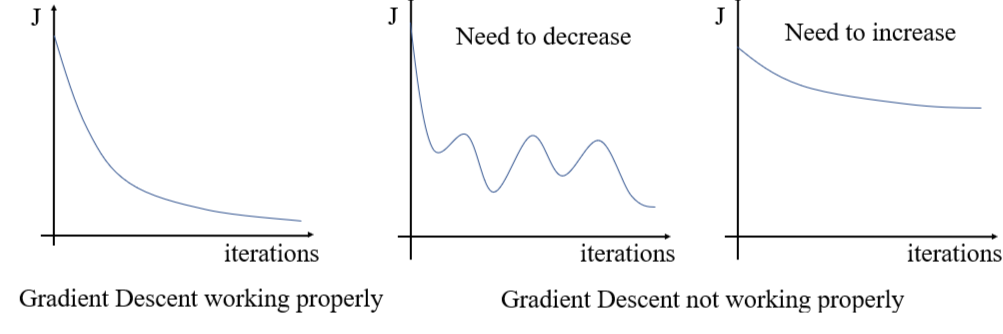
• Implementation Note-1: Choosing the value of Learning Rate α

Higher value of learning rate α, may cause Gradient Descent algorithm to oscillate around the minimum point. Too low value of αwill make Gradient Descent algorithm sluggish (i.e., too slow to converge). Hence, choosing a right value of αis important. There is no general apply-to-all value of learning rate.

As a rule of thumb to choose α people tries different values like:  …, 0.001, 0.003, 0.01, 0.03, 0.1, …

Again, this is not an exhaustive list of values of learning rate. One may choose different values like 0.005 as learning rate α.

• Implementation Note-2: Feature Scaling:

Linear Regression and most of the other Machine Learning algorithms performs well when the range of the predictor variables are roughly in the same range. This is because, if the range of one predictor variable is significantly higher than another predictor variable, then the first one starts to dominate over the second one, making Gradient Descent algorithm sluggish. Hence, Feature Scaling is necessary for faster convergence of Gradient Descent algorithm. This done by either of the following two methods.

1. Standardization: Consider a predictor variable/ feature xj whose mean is (xj) Ì… and standard deviation is σ_(x_j ), then for feature scaling replace x_j with  (x_j  -(xj) Ì…)/σ_(x_j ) , i.e.x_j  ≔(x_j  -(xj) Ì…)/σ_(x_j )  , This ensures that after scaling x_j will have zero mean and unit standard deviation.

2. Min-Max Scaling: x_j  ≔  (x_j  – (x_j ) Ì…)/(x_j^max  – x_j^min ) , This ensures that after scaling x_j will lie between -1 to +1.

Data Science Career Guide – Interview Preparation