Advanced Regression

 

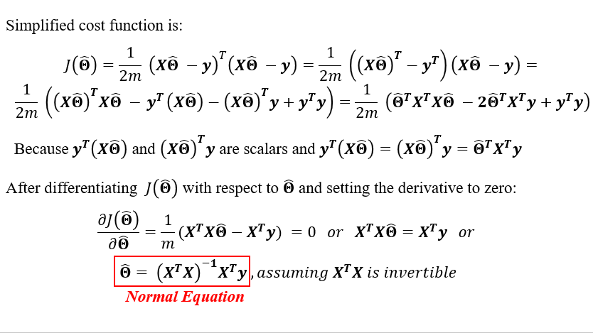
NORMAL EQUATION

 

• Gradient Descent or Normal Equation which one is preferable?

Though normal equation directly gives solution without iteration like GD, it has many drawbacks. Like, for large datasets computing (X^T X)^(-1) is a costly operation. Moreover, if X^T X is non-invertible we can’t use normal equation directly as above.

The workaround in the case when X^T X is non-invertible is to use pseudo-inverse. Hence, gradient descent is more popular and good choice for solving linear regression problem.

 

Intro to Data Science: Your Step-by-Step Guide To Starting

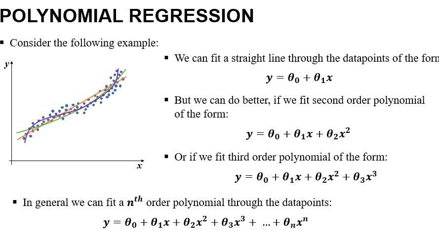
• Smaller the value of n, the complexity of the model is less but the model may not fit the dataset appropriately. So we have to choose n accordingly such that we get reasonably good fit with less complexity.

We can convert the polynomial regression problem into multiple linear regression problem just by assigning:

x1=x, x2=x2, x3=x3, …, xn=xn  and then constructing multiple linear regression model   y=θ_0+ ∑2_(i=1)^n〖θ_i x_i 〗

• For more than one predictor variables the polynomial regression becomes more complicated. For two predictor variables x_1and x_2the generalized form of second order polynomial is: y=θ_0+θ_1 x_1+θ_2 x_2+θ_3 x_1 x_2+θ_4 x_1^2+θ_5 x_2^2 

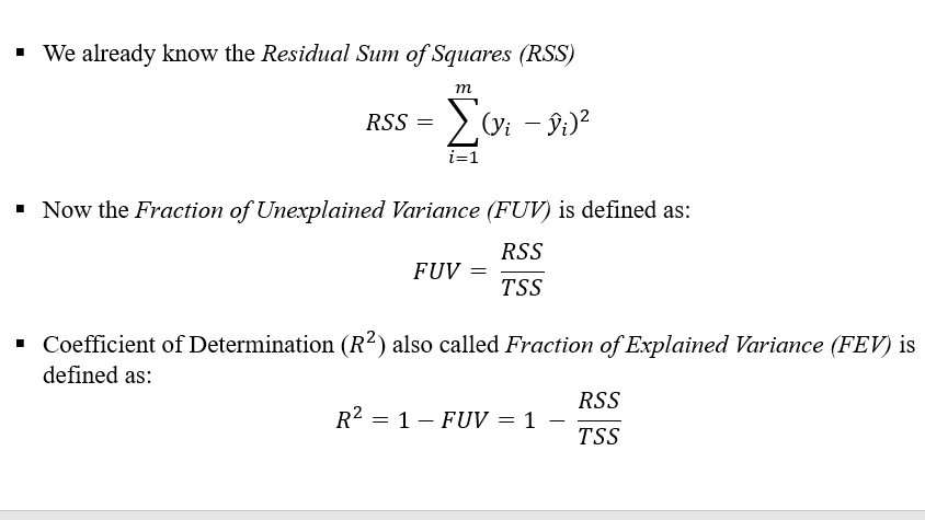
COEFFICIENT OF DETERMINATION

To determine the “goodness” of the fit in a linear regression model we use a quantitative measure. That is “Coefficient of Determination” (R^2). It is defined as follows.

Let there are m number of data points. y=[y_1, y_2, y_3, …, y_m ]^T is the vector of the actual values of target variable and y Ì‚=[y Ì‚_1, y Ì‚_2,y Ì‚_3, …, y Ì‚_m ]^T is the vector of predicted values of the target variable.

Let, y Ì… is the mean of the target variable. Then the Total Sum of Squares (TSS) is defined as follows:

TSS= ∑_(i=1)^mâ–’(y_i  – y Ì… )^2  

TSS is proportional to the variance of the target variable.

Properties of Coefficient of Determination:

• Coefficient of Determination (R^2) lies between 0 to 1
• Closer the value of R^2 to 1, Regression model fits better to our datasets and can better explain the observed variability of the target variable.
• Smaller value of R^2 implies that the regression model is not that good.
• It can be shown that for bivariate dataset

R^2=Square of the correlation coefficient between the predictor and target variable.

Cluster Analysis and Unsupervised Machine Learning in Python